Solar studies
using the mwa
Right now, the Murchison Wide-Field Array is the best imaging instrument by far for high-resolution intensity measurements done in the neighborhood the 2-meter wavelength.
By “high-resolution” I am referring to dynamic range. Dynamic range is how dark the darkest features of your image can be and how bright the brightest features of your image can be. A high dynamic range allows you to recognize finer differences or more features in your image.
Although Dr. Morales at our University of Washington uses the MWA for observation of wavelengths around 2 meters, for solar studies the MWA can also measure wavelengths from one to four meters.
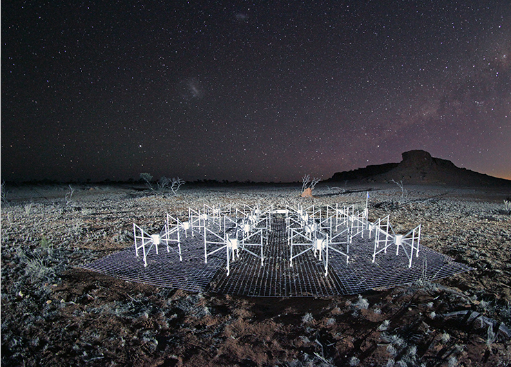
The MWA hardware is based on over four thousand antenna assemblies. The antennas are arranged in groups called “tiles”, and one tile is shown in the photograph above to the right. The photograph comes from the Murchison Wide-Field Array website, and is also copyrighted by the legal entity of the same name, Murchison Wide Field Array.
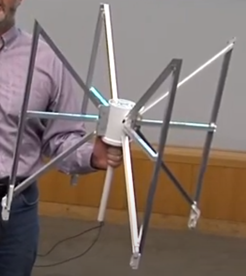
According to a published design overview, each antenna is a bowtie assembly. “Bowtie” is a technical term for this type of antenna. The bowtie assembly looks like a bacteriophage, or a spider, as shown in lower image to the right.
The bowtie antenna is a type of dipole antenna. In the single assembly photo at the right, you can see that this assembly actually has two bowties, where the two bowties form a 90-degree cross. This photo comes from a YouTube-published video lecture by Dr. Morales. This configuration is called “dual-polarization”, and serves to detect radio waves of any incident orientation. With a single polarization, the radio waves that arrive perpendicular to the bowtie would not be detected, and the radio waves that arrive with an angle close to 90 degrees relative to the bowtie would be detected only very weakly, as only its vector component that is parallel to the bowtie would be detected. Using the dual-polarized configuration ensures that all the radio waves of appropriate frequency are detected.
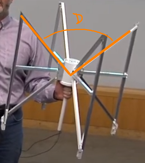
If the antenna were not a bowtie antenna, then the length of the antenna would have to be 1/2 of the wavelength that is to be detected. However, the bowtie antenna’s flared shape allows the length to be about 3/8 of the wavelength that is to be detected, according to the bowtie antenna design calculator website rfwireless-world.com . In addition to detecting the desired wavelength, the bowtie antenna can also detect other wavelengths that are close to the designed wavelength. The range of other detectable wavelengths is known as “bandwidth”, and in a bowtie antenna the bandwidth depends on the angle between the two bowtie ends. I have drawn one such angle in the image to the right, using an orange pen. I have labeled the angle as “D”. This fact comes from page 19 of a dissertation on bowtie antennas from Georgia Southern University. So this is how the Murchison array antennas are able to detect solar radio bursts from about one to four meters in wavelength.
types of solar radio bursts
type i
Type I solar radio bursts come from electrons accelerating (including just changing direction on a curved path) along magnetic field lines in the solar corona. Scientists identify these by their long duration, on the scale of hours. I think these radio waves are a type of cyclotron radiation, although this identification might be too basic for the literature to explain. Cyclotron radiation is photons that are emitted by a charged particle because it is moving in a curved or circular path defined by a magnetic field.
Type I solar radio bursts are recognizable by their rate of frequency shift. These radio waves change in frequency at rates on the order of a hundred megahertz per hour or slower.
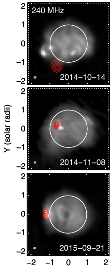
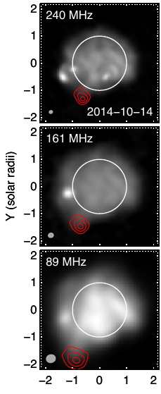
I believe that these frequency shifts are explained by random motions of magnetic field lines in the solar corona. The graph at the right shows the sun as a circle. Please disregard the red contour loops for now. The irregular white and gray shadings represent radio activity in the corona that is constant over a five-minute period. The constant radio activity is caused by thermal Bremsstrahlung radiation, which is radiation emitted by charged particles decelerating because of Coulomb repulsions with other charged particles nearby. The three snapshots in the graph show changes in the white and gray shadings, indicating changes that are slow compared to five minutes. From what I understand in my readings, such changes would cause Type I bursts. These snapshots were taken by the Murchison array. The image comes from a Murchison review paper, and this background information comes from a more general paper about solar radio bursts.
type ii
Type II solar radio bursts come from oscillations in the solar corona’s plasma, where some charges in a plasma cloud separate from the cloud by some distance a due to thermal or other excitation, and then are pulled back to the cloud by Coulomb attraction. The radiation that this acceleration of charges produces is also called Langmuir waves.
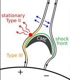
The oscillations that cause the Langmuir waves that comprise a Type II burst arise after a solar flare. They seem to be shockwaves in the bulk corona, due to the disturbance of a local solar flare. In the drawing at the right, from an article about Type II bursts, the source of a type II burst radio signal is drawn on the shockwave front of a CME, which is a Coronal Mass Ejection. The CME is like a solar flare in that it represents an explosion on the sun, but the CME is unlike a solar flare in that the CME involves an explosion of matter, while a flare involves the explosion of magnetic energy.
Type II bursts are easily distinguished from Type I bursts because the radio waves of a Type I burst change their frequency by hundreds of megahertz over several hours, while the Langmuir waves of a Type II burst change their frequency by hundreds of megahertz over several minutes.
These shifts in frequency in Langmuir waves are explained by the density gradient of the solar corona: the density of particles must be greatest near the solar surface, and lowest far from the solar surface. Plasma oscillations propagating in the high-density regions will have higher frequencies, and when they reach low-density regions their frequencies will downshift. This background information comes from a general paper about solar radio bursts .
type iii
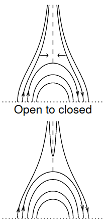
Type III solar radio bursts come from solar flare events. Specifically, the Type III burst comes from a beam of electrons that is shot straight through the corona, because of a solar flare. Even more specifically, the beam of electrons comes from the failure-to-close of magnetic field line loops: electrons are traveling along magnetic field lines, but a solar flare shoots particles outward with such energy that magnetic field lines left with loose ends instead of forming the usual closed loops. These magnetic field lines are not just flapping around in the stream of outgoing particles; instead, the field lines are actively accelerating to close, in a process called “magnetic reconnection”. I interpret the combination of magnetic reconnection and the failure-to-close as a whip-like effect, throwing charged particles out even faster than otherwise. An example of such a phenomenon is depicted in the line drawing to the left (White, 2007). Electrons traveling along those loose-end field lines escape through the corona, at very high speeds. By “very high speeds” I mean something on the order of 1/10 the speed of light. This information is inferred from the speed of the changes in wavelengths (all still in the radio range) of Langmuir waves that comprise a Type III burst. The Langmuir wavelengths depend on the density of the solar plasma. In this case, the plasma is in the corona. As the escaping electrons travel through the corona, they travel through a known density gradient. The Langmuir wavelengths increase as the plasma density decreases away from the sun, so the rate of this increase reveals the rate of the electrons’ travel.
The graph at the left shows a Type III burst in three different wavelengths, in red contour lines. The three snapshots were taken on the same day, within the same five-minute period. Each closed loop of red contour lines represents an increase in intensity by a step of 30%. Comparison of the three snapshots reveals that the higher frequency emissions come from closer to the disk of the sun (represented by the perfect, white circle), and that lower frequency emissions come from farther from the disk of the sun. This is the expected behavior of a Type III burst. These snapshots were taken by the Murchison array. They come from a Murchison review paper, and this background information comes from a more general paper about solar radio bursts.
types IV, V
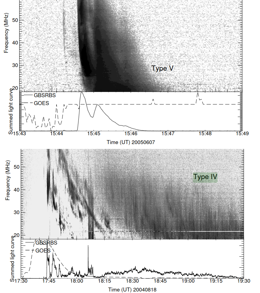
There are other solar radio bursts, including Types IV and V, but these are in wavelengths longer than the Murchison array’s capability. I gather this from two graphs in the general paper about solar radio bursts; the graphs show Type IV and Type V as below 70 MHz frequency.
a solar discovery
At this point, I have enough background knowledge to understand a couple of discoveries that the Murchison array made possible. This was published in 2019 by Dr. Mohan and his Indian research group .
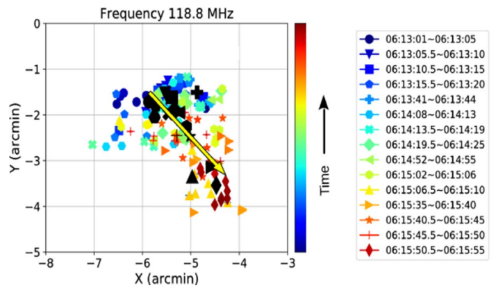
First, the better resolution (the aforementioned “dynamic range”) of the Murchison array at low frequencies (the low 100s of MHz) has allowed the Mohan group to observe a type III burst source drifting within the corona. This was done by taking multiple radio snapshots of the corona during an event that resulted in a fast series of type III bursts.
The yellow arrow shows the average direction of the drift. Each colored data point represents the location of a type III burst, and the colors proceed violet to red in order of time-of-snapshot.
Second, a little controversy has been settled by data from images from the Murchison array. The controversy was: why do type III radio bursts move around in the corona with up-and-down, almost regular (“quasi-periodic”) fluctuations in source size and source location? There have been three hypotheses: (1) the motion and fluctuations are magnetohydrodynamic effects of the interaction of the radio bursts with the corona plasma; (2) the motion and fluctuations are effects of burst radio waves triggering resonance with some particles in the corona, and knocking other particles off-resonance; (3) the motion and fluctuations are caused by some phenomenon associated with way the burst-producing electron beam entered into the corona, rather than being the result of the corona’s interaction with the radio waves of the burst.
Data from the Murchison array has narrowed down these three options to one most probable one: the third one.
Mohan et al. explain that Murchison array has been uniquely able to track the speed of the fluctuations. In fact, the fluctuations are too fast to be the result of plasma interactions with the radio burst waves, as the first two hypotheses require. The graph at the right shows area in square arc-minutes versus time in seconds. Translated into meters, the speed of these fluctuations is on the order of tens of mega-meters per second.
These are not fluctuations in frequency (such changes were already observed by cruder instruments), but these are changes in the size of the burst, that is, the area. A 50-mega-meter per second growth in either area dimension is too large to have been caused by magnetohydrodynamics in the plasma because waves of plasma in the corona only move at less than 0.3 mega-meters per second, according to McIntosh et al., 2011. These magnetohydrodynamic waves are called “Alfven waves”, and were observed by McIntosh et al. using solar telescopes (not the Murchison array). I think it is unreasonable to think that waves in a plasma can suddenly move one hundred times faster than usual, due to a beam of electrons bursting through. It is much more likely that the movement of the radio bursts is caused by something fast-moving on the solar surface, rather than by the relatively lugubrious solar plasma.
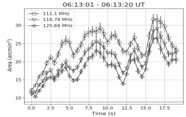
Since this website is a learning exercise, I’d like to show how to estimate the speed of source area growth. Using the circle-shaped data points (111.1 MHz) from time 0 to 2.5 seconds, I see an increase in source area of about eight square arc-minutes. Approximating the source as a square, that would be a lengthening of the side of the square by the square-root of eight (2.8) arc minutes. To estimate the length of increase in mega-meters, I use the fact that the average sun-earth distance is 93 million miles. I multiply 93 million by 1.609 km/mile, and convert to mega-meters by dividing by 1000. This sun-earth distance is the hypotenuse of a right triangle extending from Earth to the sun, whose angle on Earth is 2.8 arc-minutes. I convert the arc-minutes to radians (0.0008), and take the sine. I multiply the sine by the hypotenuse to obtain the length growth in mega-meters, and I divide by the elapsed time on the x-axis (2.5 s) to obtain about 50 mega-meters per second.
I would now like to make some comments of personal reflection.
First, I am surprised at how difficult it is to find specific information on how to calculate the dimensions of a bow-tie antenna given certain parameters of desired wavelength and desired bandwidth. I did not find any equations to match my query easily. I would like to learn more about antenna properties, and I hope that I will be empowered to do so after my physics program core course in electrodynamics.
Second, I am surprised that the direction of the drift is not exactly radial to the sun. As a layman, I just naturally think of the sun as being something from which things should radiate only outwards. Instead, the drift seems to be crossing the corona by following a longer-than-radial path (at least, along the x-axis). The Mohan group didn’t comment on that, so I conclude that the direction of the drift is not remarkable, it’s just the actual experimental observation itself of the drift that is of interest right now.
Third, I have learned in this Phys 600 unit that “magnetohydrodynamic” refers to the behavior of fluid motion caused by a fluid’s composition of charged particles subject to the influence of Coulombic and magnetic fields. This behavior is relevant because the solar corona is composed of plasma. I infer that the magnetohydrodynamics will be similar to wave motion in water or air, except that in addition to kinetic energy, the energy of the magnetohydrodynamic waves is also influenced by Coulombic forces on and among the charged particles and by any external magnetic field that the charged particles can respond to.
Fourth, I remain confused by one of the graphs in the Mohan study. It is this one:

If I try to estimate the speed of the drift, I get a speed that exceeds the speed of light by an order of magnitude. I don’t think that is possible, since these data are for the apparent drifting movement of a radio burst source. I think the speed should be much lower than the speed of light. Here’s how I do the estimate. I use just the circle-shaped data (111.1 MHz) from time=0 to time=2.5 seconds. There is a drop in position angle by 7.5 degrees. I convert to radians 0.13 radians. I multiply sun-earth distance * sin(0.13) to get the distance of drift, 19 Giga-meters, and divide by 2.5 seconds, to get 8 Gm/s. I believe I must have the wrong idea of the y-axis quantity called “relative position angle”.
Lastly, I’d like to comment on the second hypothesis that I described, about why type III bursts do quasi-periodic fluctuations in source size (area). That hypothesis was not favored by the data that the Mohan group analyzed from the Murchison array. The hypothesis was that the quasi-periodic fluctuations are the result of radio waves knocking particles on- and off-resonance in the corona. I believe the “resonance” in that hypothesis might be similar to nuclear magnetic resonance, which I know from chemistry courses. The corona has magnetic field moving around through it, and it also has charged particles. I know that nuclei have a spin, and that in the presence of an external magnetic field those spins precess at a frequency dependent on the magnetic field. I think the “resonance” that the second hypothesis occurs when burst radio waves have a frequency that matches the precession frequency of the spins of those particles. In the future I’d like to find out if this is really what is meant by “resonance” between radio waves and plasma particles in the solar corona.
Thank you for your time, Dr. Wilkes.